15.2 Case Study: Classification with k-Nearest Neighbors and the Digits Dataset, Part 1
- To process mail efficiently and route each letter to the correct destination, postal service computers must be able to scan handwritten names, addresses and zip codes and recognize the letters and digits
- Scikit-learn enables even novice programmers to make such machine-learning problems manageable
Supervised Machine Learning: Classification
- Attempt to predict the distinct class (category) to which a sample belongs
- Binary classification—two classes (e.g., “dog” or “cat”)
- Digits dataset bundled with scikit-learn
- 8-by-8 pixel images representing 1797 hand-written digits (0 through 9)
- Goal: Predict which digit an image represents
- Multi-classification—10 possible digits (the classes)
- Train a classification model using labeled data—know in advance each digit’s class
- We’ll use one of the simplest machine-learning classification algorithms, k-nearest neighbors (k-NN), to recognize handwritten digits
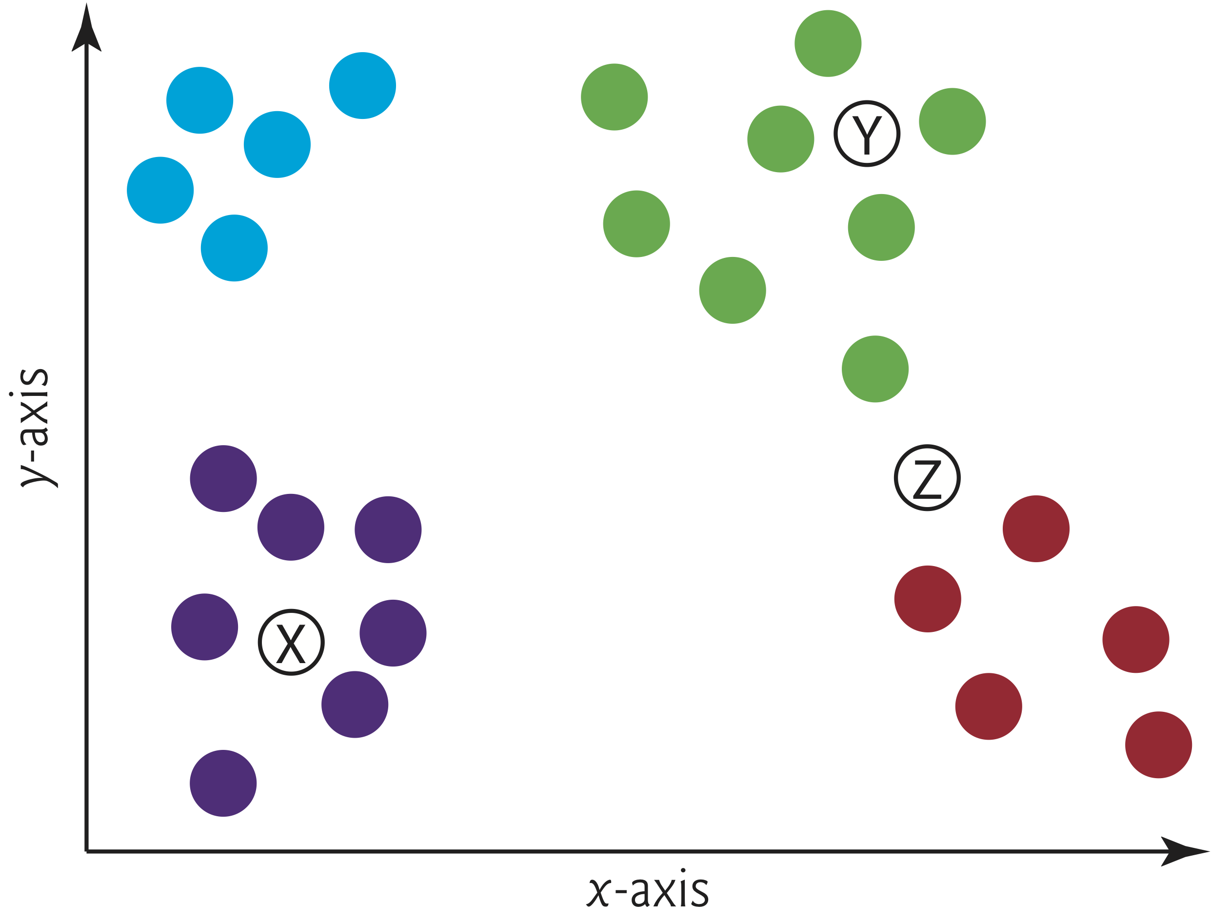
15.2.1 k-Nearest Neighbors Algorithm (k-NN)
- Predict a sample’s class by looking at the k training samples nearest in "distance" to the sample
- Filled dots represent four distinct classes—A (blue), B (green), C (red) and D (purple)
- Class with the most “votes” wins
- Odd k value avoids ties — there’s never an equal number of votes
15.2.2 Loading the Dataset with the load_digits Function
- Returns a
Bunchobject containing digit samples and metadata - A
Bunchis a dictionary with additional dataset-specific attributes
from sklearn.datasets import load_digits
digits = load_digits()
Displaying Digits Dataset's Description
- Digits dataset is a subset of the UCI (University of California Irvine) ML hand-written digits dataset
- Original dataset: 5620 samples—3823 for training and 1797 for testing
- Digits dataset: Only the 1797 testing samples
- A Bunch’s
DESCRattribute contains dataset's description- Each sample has
64features (Number of Attributes) that represent an 8-by-8 image with pixel values0–16(Attribute Information) - No missing values (
Missing Attribute Values)
- Each sample has
- 64 features may seem like a lot
- Datasets can have hundreds, thousands or even millions of features
- Processing datasets like these can require enormous computing capabilities
print(digits.DESCR)
type(digits)
Dictionary-like object, the interesting attributes are: ‘data’, the data to learn, ‘images’, the images corresponding to each sample, ‘target’, the classification labels for each sample, ‘target_names’, the meaning of the labels, and ‘DESCR’, the full description of the dataset.
The input data can be accessed by:
digits.data
The target variable data can be accessed by:
digits.target
Checking the Sample and Target Sizes (1 of 2)
Bunchobject’sdataandtargetattributes are NumPy arrays:dataarray: The 1797 samples (digit images), each with 64 features with values 0 (white) to 16 (black), representing pixel intensities to black (16)")
targetarray: The images’ labels, (classes) indicating which digit each image represents
digits.target[::100] # target values of every 100th sample
Remember:
The slicing parameters are aptly named
slice[start:stop:step]so the slice starts at the location defined by start, stops before the location stop is reached, and moves from one position to the next by step items.
>>> "ABCD"[0:4:2]
'AC'
Checking the Sample and Target Sizes (2 of 2)
- Confirm number of samples and features (per sample) via
dataarray’sshape
digits.data.shape
- Confirm that number of target values matches number of samples via
targetarray’sshape
digits.target.shape
digits.data
digits.data[0]
digits.target[0]
digits.data[1]
digits.target[0],digits.target[1]
A Sample Digit Image
- Images are two-dimensional—width and a height in pixels
- Digits dataset's
Bunchobject has animagesattribute- Each element is an 8-by-8 array representing a digit image’s pixel intensities
- Scikit-learn stores the intensity values as NumPy type
float64
digits.images[13] # show array for sample image at index 13
Visualization of
digits.images[13]
digits.target[0],digits.target[1], digits.target[13]
import matplotlib.pyplot as plt
plt.gray()
plt.matshow(digits.images[0])
plt.show()

digits.data[0]
import matplotlib.pyplot as plt
plt.gray()
plt.matshow(digits.images[1])
plt.show()

import matplotlib.pyplot as plt
plt.gray()
plt.matshow(digits.images[13])
plt.show()

Preparing the Data for Use with Scikit-Learn (1 of 2)
- Scikit-learn estimators require samples to be stored in a two-dimensional array of floating-point values (or list of lists or pandas
DataFrame):- Each row represents one sample
- Each column in a given row represents one feature for that sample
- Multi-dimensional data samples must be flattened into a one-dimensional array
- For categorical features (e.g., strings like
'spam'or'not-spam'), you’d have to preprocess those features into numerical values—known as one-hot encoding (discussed later in deep learning)
Preparing the Data for Use with Scikit-Learn (2 of 2)
load_digitsreturns the preprocessed data ready for machine learning- 8-by-8 array
digits.images[13]corresponds to 1-by-64 arraydigits.data[13]:
digits.data[13]
15.2.3 Visualizing the Data (1 of 2)
- Always familiarize yourself with your data—called data exploration
- Let's visualize the dataset’s first 24 images with Matplotlib
- To see how difficult a problem handwritten digit recognition is, consider the variations among the images of the 3s in the first, third and fourth rows, and look at the images of the 2s in the first, third and fourth rows.
15.2.3 Visualizing the Data (2 of 2)
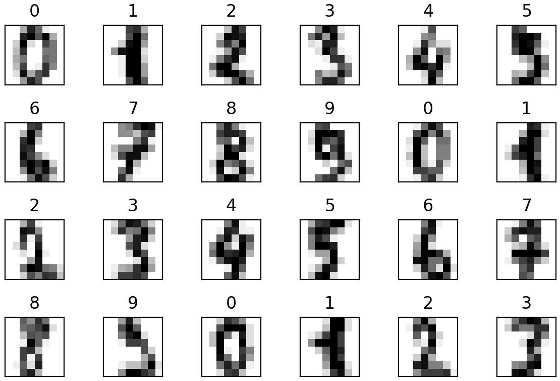
Creating the Diagram
- Color map
plt.cm.gray_ris for grayscale with 0 for white - Matplotlib’s color map names—accessible via
plt.cmobject or a string, like'gray_r'
import matplotlib.pyplot as plt
figure, axes = plt.subplots(nrows=4, ncols=6, figsize=(6, 4))

for item in zip(axes.ravel(), digits.images, digits.target):
    axes, image, target = item
    axes.imshow(image, cmap=plt.cm.gray_r)
    axes.set_xticks([])  # remove x-axis tick marks
    axes.set_yticks([])  # remove y-axis tick marks
    axes.set_title(target)
plt.tight_layout()

15.2.4 Splitting the Data for Training and Testing (1 of 2)
- Typically train a model with a subset of a dataset
- Save a portion for testing, so you can evaluate a model’s performance using unseen data
- Function
train_test_splitshuffles the data to randomize it, then splits the samples in thedataarray and the target values in thetargetarray into training and testing sets- Shuffling helps ensure that the training and testing sets have similar characteristics
- Returns a tuple of four elements in which the first two are the samples split into training and testing sets, and the last two are the corresponding target values split into training and testing sets
15.2.4 Splitting the Data for Training and Testing (2 of 2)
- Convention:
- Uppercase
Xrepresents samples - Lowercase
yrepresents target values
- Uppercase
from sklearn.model_selection import train_test_split
X_train, X_test, y_train, y_test = train_test_split(
    digits.data, digits.target, random_state=11)  # random_state for reproducibility
- Scikit-learn bundled classification datasets have balanced classes
- Samples are divided evenly among the classes
- Unbalanced classes could lead to incorrect results
Training and Testing Set Sizes
- By default,
train_test_splitreserves 75% of the data for training and 25% for testing- See how to customize this in my Python Fundamentals LiveLessons videos or in Python for Programmers, Section 14.2.4
X_train.shape
X_test.shape
15.2.5 Creating the Model
- In scikit-learn, models are called estimators
KNeighborsClassifierestimator implements the k-nearest neighbors algorithm
from sklearn.neighbors import KNeighborsClassifier
knn = KNeighborsClassifier()
15.2.6 Training the Model with the KNeighborsClassifier Object’s fit method (1 of 2)
- Load sample training set (
X_train) and target training set (y_train) into the estimator
knn.fit(X=X_train, y=y_train)
n_neighborscorresponds to k in the k-nearest neighbors algorithmKNeighborsClassifierdefault settings
15.2.6 Training the Model with the KNeighborsClassifier Object’s fit method (2 of 2)
fitnormally loads data into an estimator then performs complex calculations behind the scenes that learn from the data to train a modelKNeighborsClassifier’sfitmethod just loads the data- No initial learning process
- The estimator is lazy — work is performed only when you use it to make predictions
- Lots of models have significant training phases that can take minutes, hours, days or more
- High-performance GPUs and TPUs can significantly reduce model training time
15.2.7 Predicting Digit Classes with the KNeighborsClassifier’s predict method (1 of 2)
- Returns an array containing the predicted class of each test image:
predicted = knn.predict(X=X_test)
expected = y_test
predicteddigits vs.expecteddigits for the first 20 test samples—see index 18
predicted[:20]
expected[:20]
15.2.7 Predicting Digit Classes with the KNeighborsClassifier’s predict method (2 of 2)
- Locate all incorrect predictions for the entire test set:
wrong = [(p, e) for (p, e) in zip(predicted, expected) if p != e]
wrong
- Incorrectly predicted only 10 of the 450 test samples
15.3 Case Study: Classification with k-Nearest Neighbors and the Digits Dataset, Part 2
15.3.1 Metrics for Measuring Model Accuracy
Estimator Method score
- Returns an indication of how well the estimator performs on test data
- For classification estimators, returns the prediction accuracy for the test data:
print(f'{knn.score(X_test, y_test):.2%}')
kNeighborsClassifierwith default k of 5 achieved 97.78% prediction accuracy using only the estimator’s default parameters- Can use hyperparameter tuning to try to determine the optimal value for k
Confusion Matrix (1 of 2)
- Shows correct and incorrect predicted values (the hits and misses) for a given class
from sklearn.metrics import confusion_matrix
confusion = confusion_matrix(y_true=expected, y_pred=predicted)
confusion
Confusion Matrix (2 of 2)
- Correct predictions shown on principal diagonal from top-left to bottom-right
- Nonzero values not on principal diagonal indicate incorrect predictions
- Each row represents one distinct class (0–9)
- Columns specify how many test samples were classified into classes 0–9
- Row 0 shows digit class
0—all 0s were predicted correctly[45, 0, 0, 0, 0, 0, 0, 0, 0, 0] Row 8 shows digit class
8—five 8s were predicted incorrectly[ 0, 1, 1, 2, 0, 0, 0, 0, 39, 1]- Correctly predicted 88.63% (39 of 44) of
8s - 8s harder to recognize
- Correctly predicted 88.63% (39 of 44) of
Visualizing the Confusion Matrix
- A heat map displays values as colors
- Convert the confusion matrix into a
DataFrame, then graph it - Principal diagonal and incorrect predictions stand out nicely in heat map
import pandas as pd
confusion_df = pd.DataFrame(confusion, index=range(10), columns=range(10))
import seaborn as sns
figure = plt.figure(figsize=(7, 6))
axes = sns.heatmap(confusion_df, annot=True,
                   cmap=plt.cm.nipy_spectral_r)

15.3.2 K-Fold Cross-Validation
- Uses all of your data for training and testing
- Gives a better sense of how well your model will make predictions
- Splits the dataset into k equal-size folds (unrelated to k in the k-nearest neighbors algorithm)
- Repeatedly trains your model with k – 1 folds and test the model with the remaining fold
- Consider using k = 10 with folds numbered 1 through 10
- train with folds 1–9, then test with fold 10
- train with folds 1–8 and 10, then test with fold 9
- train with folds 1–7 and 9–10, then test with fold 8
- ...
KFold Class
KFoldclass and functioncross_val_scoreperform k-fold cross validationn_splits=10specifies the number of foldsshuffle=Truerandomizes the data before splitting it into folds- Particularly important if the samples might be ordered or grouped (as in Iris dataset we'll see later)
from sklearn.model_selection import KFold
kfold = KFold(n_splits=10, random_state=11, shuffle=True)
Calling Function cross_val_score to Train and Test Your Model (1 of 2)
estimator=knn— estimator to validateX=digits.data— samples to use for training and testingy=digits.target— target predictions for the samplescv=kfold— cross-validation generator that defines how to split the samples and targets for training and testing
from sklearn.model_selection import cross_val_score
scores = cross_val_score(estimator=knn, X=digits.data, y=digits.target, cv=kfold)
Calling Function cross_val_score to Train and Test Your Model (2 of 2)
- Lowest accuracy was 97.78% — one was 100%
scores # array of accuracy scores for each fold
print(f'Mean accuracy: {scores.mean():.2%}')
- Mean accuracy even better than the 97.78% we achieved when we trained the model with 75% of the data and tested the model with 25% earlier
15.3.3 Running Multiple Models to Find the Best One (1 of 3)
- Difficult to know in advance which machine learning model(s) will perform best for a given dataset
- Especially when they hide the details of how they operate
- Even though the
KNeighborsClassifierpredicts digit images with a high degree of accuracy, it’s possible that other estimators are even more accurate - Let’s compare
KNeighborsClassifier,SVCandGaussianNB
15.3.3 Running Multiple Models to Find the Best One (2 of 3)
from sklearn.svm import SVC
from sklearn.naive_bayes import GaussianNB
- Create the estimators
- To avoid a scikit-learn warning, we supplied a keyword argument when creating the
SVCestimator- This argument’s value will become the default in scikit-learn version 0.22
estimators = {
    'KNeighborsClassifier': knn,
    'SVC': SVC(gamma='scale'),
    'GaussianNB': GaussianNB()}
15.3.3 Running Multiple Models to Find the Best One (3 of 3)
- Execute the models:
for estimator_name, estimator_object in estimators.items():
    kfold = KFold(n_splits=10, random_state=11, shuffle=True)
    scores = cross_val_score(estimator=estimator_object,
        X=digits.data, y=digits.target, cv=kfold)
    print(f'{estimator_name:>20}: ' +
          f'mean accuracy={scores.mean():.2%}; ' +
          f'standard deviation={scores.std():.2%}')
KNeighborsClassifierandSVCestimators’ accuracies are identical so we might want to perform hyperparameter tuning on each to determine the best
15.3.4 Hyperparameter Tuning (1 of 3)
- In real-world machine learning studies, you’ll want to tune hyperparameters to choose values that produce the best possible predictions
- To determine the best value for k in the kNN algorithm, try different values and compare performance
- Scikit-learn also has automated hyperparameter tuning capabilities
15.3.4 Hyperparameter Tuning (2 of 3)
- Create
KNeighborsClassifierswith odd k values from 1 through 19 - Perform k-fold cross-validation on each
for k in range(1, 20, 2):  # k is an odd value 1-19; odds prevent ties
    kfold = KFold(n_splits=10, random_state=11, shuffle=True)
    knn = KNeighborsClassifier(n_neighbors=k)
    scores = cross_val_score(estimator=knn,
        X=digits.data, y=digits.target, cv=kfold)
    print(f'k={k:<2}; mean accuracy={scores.mean():.2%}; ' +
          f'standard deviation={scores.std():.2%}')
15.3.4 Hyperparameter Tuning (3 of 3)
- Machine learning is not without its costs, especially in big data and deep learning
- Compute time grows rapidly with k, because k-NN needs to perform more calculations to find the nearest neighbors
- Can use function
cross_validateto perform cross-validation and time the results
©1992–2020 by Pearson Education, Inc. All Rights Reserved. This content is based on Chapter 5 of the book Intro to Python for Computer Science and Data Science: Learning to Program with AI, Big Data and the Cloud.
DISCLAIMER: The authors and publisher of this book have used their best efforts in preparing the book. These efforts include the development, research, and testing of the theories and programs to determine their effectiveness. The authors and publisher make no warranty of any kind, expressed or implied, with regard to these programs or to the documentation contained in these books. The authors and publisher shall not be liable in any event for incidental or consequential damages in connection with, or arising out of, the furnishing, performance, or use of these programs.