15.7 Case Study: Unsupervised Machine Learning, Part 2—k-Means Clustering (1 of 2)

• Simplest unsupervised machine learning algorithm
• Analyze unlabeled samples and attempt to place them in clusters
• k hyperparameter represents number of clusters to impose on the data
• Organizes clusters using distance calculations similar to the k-NN classification

15.7 Case Study: Unsupervised Machine Learning, Part 2—k-Means Clustering (2 of 2)

• Each cluster is grouped around a centroid (cluster’s center point)
• Initially, the algorithm chooses k centroids at random from dataset’s samples
• Remaining samples placed in the cluster whose centroid is the closest
• Centroids are iteratively recalculated and samples re-assigned to clusters until, for all clusters, distances from a given centroid to the samples in its cluster are minimized Results are:
  • one-dimensional array of labels indicating cluster to which each sample belongs
  • two-dimensional array of clusters' centroids

Iris Dataset

• Iris dataset — commonly analyzed with classification and clustering
  • Fisher, R.A., “The use of multiple measurements in taxonomic problems,” Annual Eugenics, 7, Part II, 179-188 (1936); also in “Contributions to Mathematical Statistics” (John Wiley, NY, 1950).
• Dataset is labeled — we’ll ignore labels to demonstrate clustering
  • Use labels later to determine how well k-means algorithm clustered samples
• "Toy dataset" — has only 150 samples and four features
  • 50 samples for each of three Iris flower species (balanced classes)
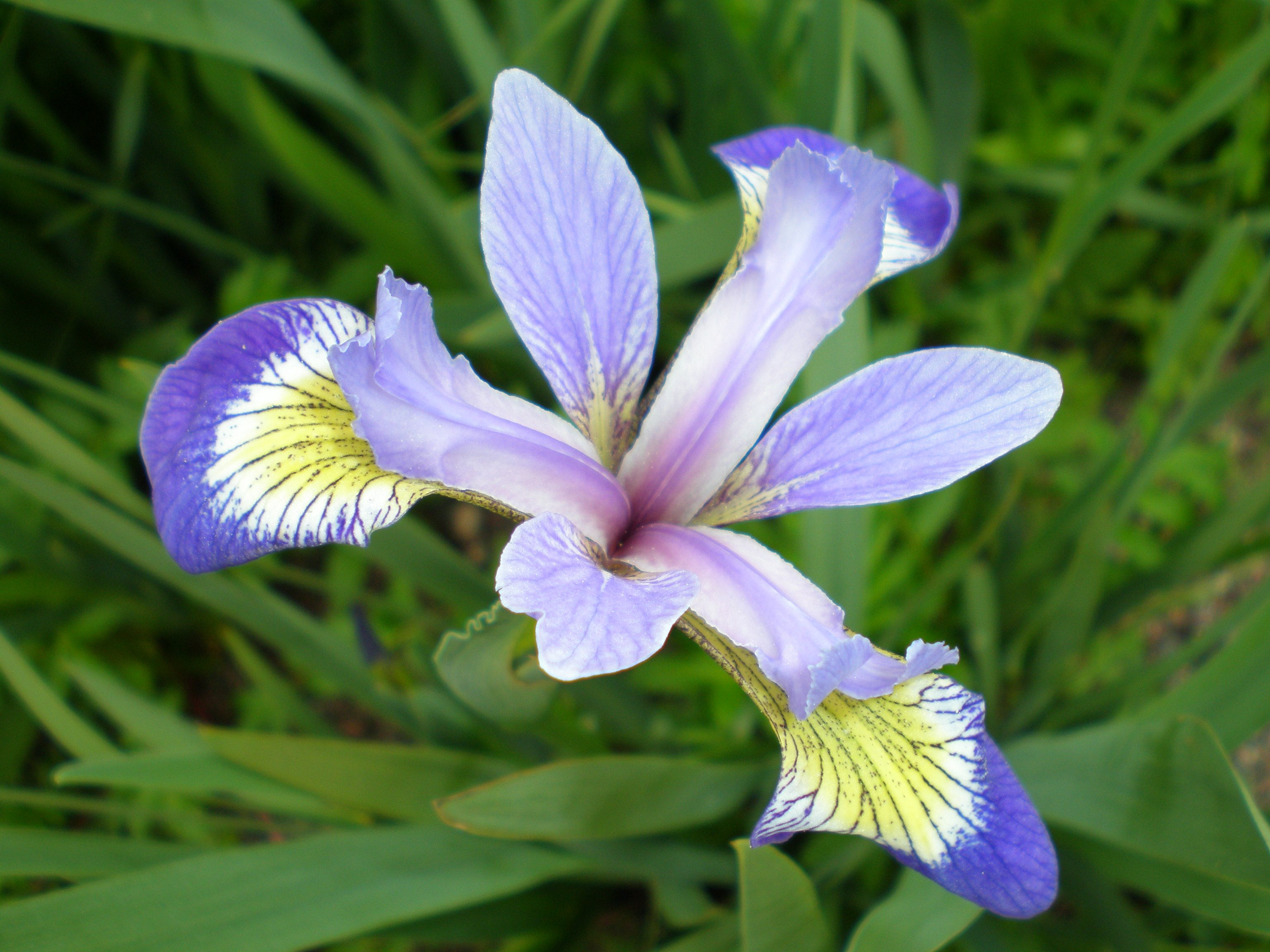
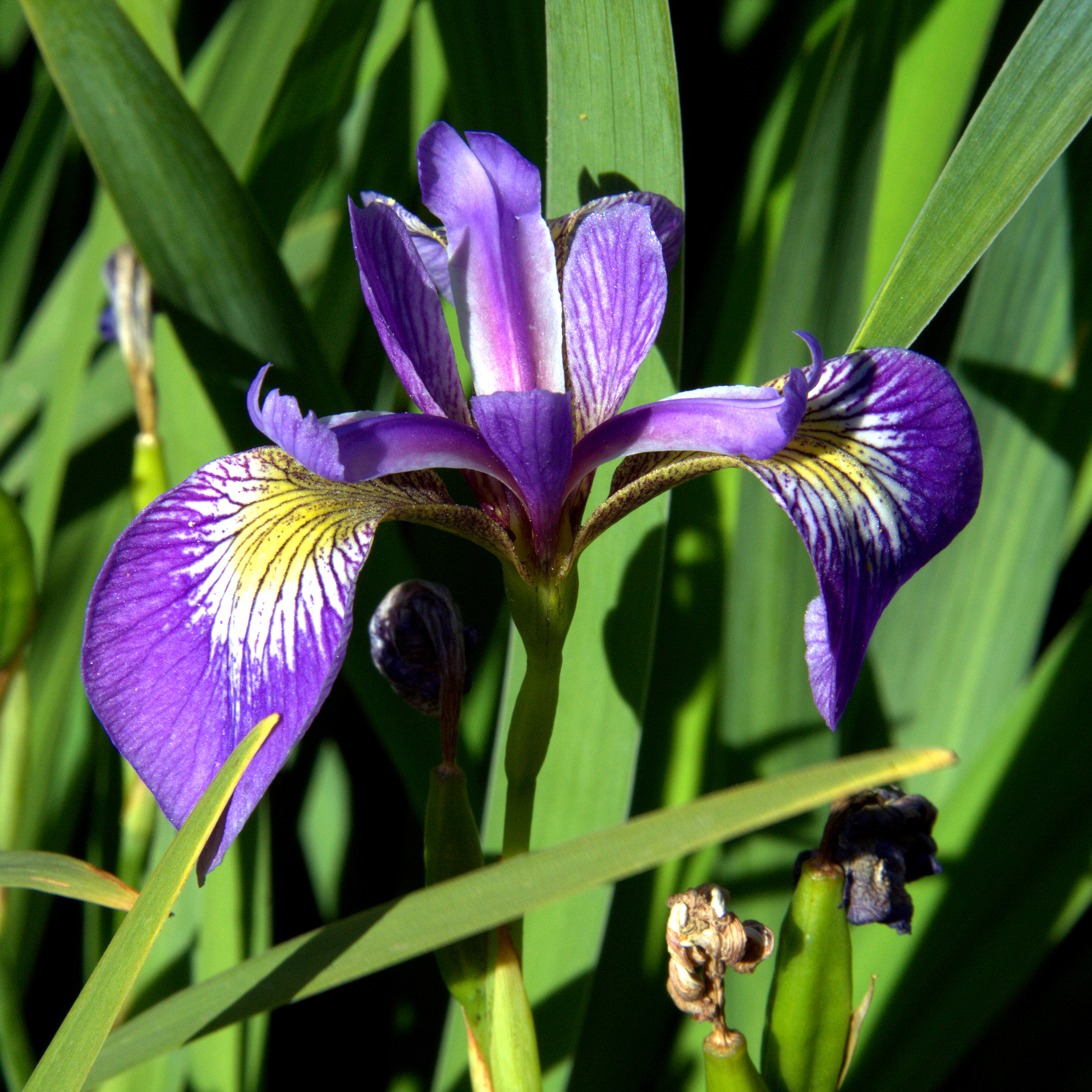
  • Iris setosa, Iris versicolor and Iris virginica
  • Features: sepal length, sepal width, petal length and petal width, all measured in centimeters.
  • Sepals are larger outer parts of each flower that protect smaller inside petals before buds bloom

Iris setosa: https://commons.wikimedia.org/wiki/File:Wild_iris_KEFJ_(9025144383).jpg. Credit: Courtesy of Nation Park services.

Iris versicolor: https://commons.wikimedia.org/wiki/Iris_versicolor#/media/File:IrisVersicolor-FoxRoost-Newfoundland.jpg. Credit: Courtesy of Jefficus, https://commons.wikimedia.org/w/index.php?title=User:Jefficus&action=edit&redlink=1

Iris virginica: https://commons.wikimedia.org/wiki/File:IMG_7911-Iris_virginica.jpg. Credit: Christer T Johansson.

15.7.1 Loading the Iris Dataset

• Classifies samples by labeling them with the integers 0, 1 and 2, representing Iris setosa, Iris versicolor and Iris virginica, respectively

from sklearn.datasets import load_iris

iris = load_iris()

print(iris.DESCR)

.. _iris_dataset:

Iris plants dataset
--------------------

**Data Set Characteristics:**

    :Number of Instances: 150 (50 in each of three classes)
    :Number of Attributes: 4 numeric, predictive attributes and the class
    :Attribute Information:
        - sepal length in cm
        - sepal width in cm
        - petal length in cm
        - petal width in cm
        - class:
                - Iris-Setosa
                - Iris-Versicolour
                - Iris-Virginica
                
    :Summary Statistics:

    ============== ==== ==== ======= ===== ====================
                    Min  Max   Mean    SD   Class Correlation
    ============== ==== ==== ======= ===== ====================
    sepal length:   4.3  7.9   5.84   0.83    0.7826
    sepal width:    2.0  4.4   3.05   0.43   -0.4194
    petal length:   1.0  6.9   3.76   1.76    0.9490  (high!)
    petal width:    0.1  2.5   1.20   0.76    0.9565  (high!)
    ============== ==== ==== ======= ===== ====================

    :Missing Attribute Values: None
    :Class Distribution: 33.3% for each of 3 classes.
    :Creator: R.A. Fisher
    :Donor: Michael Marshall (MARSHALL%PLU@io.arc.nasa.gov)
    :Date: July, 1988

The famous Iris database, first used by Sir R.A. Fisher. The dataset is taken
from Fisher's paper. Note that it's the same as in R, but not as in the UCI
Machine Learning Repository, which has two wrong data points.

This is perhaps the best known database to be found in the
pattern recognition literature.  Fisher's paper is a classic in the field and
is referenced frequently to this day.  (See Duda & Hart, for example.)  The
data set contains 3 classes of 50 instances each, where each class refers to a
type of iris plant.  One class is linearly separable from the other 2; the
latter are NOT linearly separable from each other.

.. topic:: References

   - Fisher, R.A. "The use of multiple measurements in taxonomic problems"
     Annual Eugenics, 7, Part II, 179-188 (1936); also in "Contributions to
     Mathematical Statistics" (John Wiley, NY, 1950).
   - Duda, R.O., & Hart, P.E. (1973) Pattern Classification and Scene Analysis.
     (Q327.D83) John Wiley & Sons.  ISBN 0-471-22361-1.  See page 218.
   - Dasarathy, B.V. (1980) "Nosing Around the Neighborhood: A New System
     Structure and Classification Rule for Recognition in Partially Exposed
     Environments".  IEEE Transactions on Pattern Analysis and Machine
     Intelligence, Vol. PAMI-2, No. 1, 67-71.
   - Gates, G.W. (1972) "The Reduced Nearest Neighbor Rule".  IEEE Transactions
     on Information Theory, May 1972, 431-433.
   - See also: 1988 MLC Proceedings, 54-64.  Cheeseman et al"s AUTOCLASS II
     conceptual clustering system finds 3 classes in the data.
   - Many, many more ...

Checking the Numbers of Samples, Features and Targets

• Array target_names contains names for the target array’s numeric labels
• dtype='<U10' — elements are strings with a max of 10 characters
• feature_names contains names for each column in the data array

iris.data.shape

(150, 4)

iris.target.shape

(150,)

iris.target

array([0, 0, 0, 0, 0, 0, 0, 0, 0, 0, 0, 0, 0, 0, 0, 0, 0, 0, 0, 0, 0, 0,
       0, 0, 0, 0, 0, 0, 0, 0, 0, 0, 0, 0, 0, 0, 0, 0, 0, 0, 0, 0, 0, 0,
       0, 0, 0, 0, 0, 0, 1, 1, 1, 1, 1, 1, 1, 1, 1, 1, 1, 1, 1, 1, 1, 1,
       1, 1, 1, 1, 1, 1, 1, 1, 1, 1, 1, 1, 1, 1, 1, 1, 1, 1, 1, 1, 1, 1,
       1, 1, 1, 1, 1, 1, 1, 1, 1, 1, 1, 1, 2, 2, 2, 2, 2, 2, 2, 2, 2, 2,
       2, 2, 2, 2, 2, 2, 2, 2, 2, 2, 2, 2, 2, 2, 2, 2, 2, 2, 2, 2, 2, 2,
       2, 2, 2, 2, 2, 2, 2, 2, 2, 2, 2, 2, 2, 2, 2, 2, 2, 2])

iris.target_names

array(['setosa', 'versicolor', 'virginica'], dtype='<U10')

iris.feature_names

['sepal length (cm)',
 'sepal width (cm)',
 'petal length (cm)',
 'petal width (cm)']

15.7.2 Exploring the Iris Dataset: Descriptive Statistics with a Pandas

import pandas as pd

# pd.set_option('max_columns', 5)  # needed only in IPython interactive mode

# pd.set_option('display.width', None)  # needed only in IPython interactive mode

• Create a DataFrame containing the data array’s contents
• Use feature_names as the column names

iris_df = pd.DataFrame(iris.data, columns=iris.feature_names)

• Add a column containing each sample’s species name
• List comprehension uses each value in target array to look up the corresponding species name in target_names array

iris_df['species'] = [iris.target_names[i] for i in iris.target]

• Look at a few samples

iris_df.head()

	sepal length (cm)	sepal width (cm)	petal length (cm)	petal width (cm)	species
0	5.1	3.5	1.4	0.2	setosa
1	4.9	3.0	1.4	0.2	setosa
2	4.7	3.2	1.3	0.2	setosa
3	4.6	3.1	1.5	0.2	setosa
4	5.0	3.6	1.4	0.2	setosa

• Calculate descriptive statistics on the numeric columns

pd.set_option('precision', 2)

iris_df.describe()

	sepal length (cm)	sepal width (cm)	petal length (cm)	petal width (cm)
count	150.00	150.00	150.00	150.00
mean	5.84	3.06	3.76	1.20
std	0.83	0.44	1.77	0.76
min	4.30	2.00	1.00	0.10
25%	5.10	2.80	1.60	0.30
50%	5.80	3.00	4.35	1.30
75%	6.40	3.30	5.10	1.80
max	7.90	4.40	6.90	2.50

• Calling describe on the 'species' column confirms that it contains three unique values

iris_df['species'].describe()

count           150
unique            3
top       virginica
freq             50
Name: species, dtype: object

• We know in advance that there are three classes to which the samples belong
  • This is not typically the case in unsupervised machine learning

15.7.3 Visualizing the Dataset with a Seaborn pairplot

• To learn more about your data, visualize how the features relate to one another
• Four features — cannot graph one against other three in a single graph
• Can plot pairs of features against one another
• Seaborn function pairplot creates a grid of graphs

import seaborn as sns

# sns.set(font_scale=1.1)

sns.set_style('whitegrid')

grid = sns.pairplot(data=iris_df, vars=iris_df.columns[0:4], hue='species')

15.7.3 Visualizing the Dataset with a Seaborn pairplot (cont.)

• The keyword arguments are:
  • data—The DataFrame (or two-dimensional array or list) containing the data to plot.
  • vars—A sequence containing the names of the variables to plot. For a DataFrame, these are the names of the columns to plot. Here, we use the first four DataFrame columns, representing the sepal length, sepal width, petal length and petal width, respectively.
  • hue—The DataFrame column that’s used to determine colors of the plotted data. In this case, we’ll color the data by Iris species.

15.7.3 Visualizing the Dataset with a Seaborn pairplot (cont.)

• The graphs along the top-left-to-bottom-right diagonal, show the distribution of just the feature plotted in that column, with the range of values (left-to-right) and the number of samples with those values (top-to-bottom).
• Other graphs in a column show scatter plots of the other features against the feature on the x-axis.
• Interestingly, all the scatter plots clearly separate the Iris setosa blue dots from the other species’ orange and green dots, indicating that Iris setosa is indeed in a “class by itself.”
• The other two species can sometimes be confused with one another, as indicated by the overlapping orange and green dots.
  • It would be difficult to distinguish between these two species if we had only the sepal measurements available to us.

Displaying the pairplot in One Color

• If you remove the hue keyword argument, pairplot uses only one color to plot all the data because it does not know how to distinguish the species:

grid = sns.pairplot(data=iris_df, vars=iris_df.columns[0:4])

Displaying the pairplot in One Color (cont.)

• In this case, the graphs along the diagonal are histograms showing the distributions of all the values for that feature, regardless of the species.
• It appears that there may be only two distinct clusters, even though for this dataset we know there are three species.
  • If you do not know the number of clusters in advance, you might ask a domain expert who is thoroughly familiar with the data.
  • Such a person might know that there are three species in the dataset, which would be valuable information as we try to perform machine learning on the data.
• The pairplot diagrams work well for a small number of features or a subset of features so that you have a small number of rows and columns, and for a relatively small number of samples so you can see the data points.
• As the number of features and samples increases, each scatter plot quickly becomes too small to read.

15.7.4 Using a KMeans Estimator

• Use k-means clustering via KMeans estimator to place each sample in the Iris dataset into a cluster

Creating the KMeans Estimator

• KMeans default arguments
• When you train a KMeans estimator, it calculates for each cluster a centroid representing the cluster’s center data point
  • Often, you’ll rely on domain experts to help choose an appropriate k (n_clusters).
• Can also use hyperparameter tuning to estimate the appropriate k

from sklearn.cluster import KMeans

kmeans = KMeans(n_clusters=3, random_state=11)

Fitting the Model Via the KMeans object’s fit Method

• When the training completes, the KMeans object contains:
  • labels_ array with values from 0 to n_clusters - 1, indicating the clusters to which the samples belong
  • cluster_centers_ array in which each row represents a centroid

kmeans.fit(iris.data)

KMeans(algorithm='auto', copy_x=True, init='k-means++', max_iter=300,
       n_clusters=3, n_init=10, n_jobs=None, precompute_distances='auto',
       random_state=11, tol=0.0001, verbose=0)

Comparing the Cluster Labels to the Iris Dataset’s Target Values

• Iris dataset is labeled, so we can look at target array values to get a sense of how well the k-means algorithm clustered the samples
  • With unlabeled data, we’d depend on a domain expert to help evaluate whether the predicted classes make sense
• First 50 samples are Iris setosa, next 50 are Iris versicolor, last 50 are Iris virginica
  • target array represents these with values 0–2
• If KMeans chose clusters perfectly, then each group of 50 elements in the estimator’s labels_ array should have a distinct label.
  • KMeans labels are not related to dataset’s target array

Comparing the Cluster Labels to the Iris Dataset’s Target Values (cont.)

• First 50 samples should be one cluster

print(kmeans.labels_[0:50])

[1 1 1 1 1 1 1 1 1 1 1 1 1 1 1 1 1 1 1 1 1 1 1 1 1 1 1 1 1 1 1 1 1 1 1 1 1
 1 1 1 1 1 1 1 1 1 1 1 1 1]

• Next 50 samples should be a second cluster (two are not)

print(kmeans.labels_[50:100])

[0 0 2 0 0 0 0 0 0 0 0 0 0 0 0 0 0 0 0 0 0 0 0 0 0 0 0 2 0 0 0 0 0 0 0 0 0
 0 0 0 0 0 0 0 0 0 0 0 0 0]

• Last 50 samples should be a third cluster (14 are not)

print(kmeans.labels_[100:150])

[2 0 2 2 2 2 0 2 2 2 2 2 2 0 0 2 2 2 2 0 2 0 2 0 2 2 0 0 2 2 2 2 2 0 2 2 2
 2 0 2 2 2 0 2 2 2 0 2 2 0]

• Results confirm what we saw in pairplot diagrams
  • Iris setosa is “in a class by itself”
  • There is confusion between Iris versicolor and Iris virginica

15.7.5 Dimensionality Reduction with Principal Component Analysis

• Use PCA estimator to perform dimensionality reduction from 4 to 2 dimensions
  • Algorithm’s details beyond scope

from sklearn.decomposition import PCA

pca = PCA(n_components=2, random_state=11)

Transforming the Iris Dataset’s Features into Two Dimensions

pca.fit(iris.data)  # trains estimator once

PCA(copy=True, iterated_power='auto', n_components=2, random_state=11,
    svd_solver='auto', tol=0.0, whiten=False)

iris_pca = pca.transform(iris.data)  # can be called many times to reduce data

• We'll call transform again to reduce the cluster centroids from four dimensions to two for plotting
• transform returns an array with same number of rows as iris.data, but only two columns

iris_pca[0:5,:]

array([[-2.68412563,  0.31939725],
       [-2.71414169, -0.17700123],
       [-2.88899057, -0.14494943],
       [-2.74534286, -0.31829898],
       [-2.72871654,  0.32675451]])

iris_pca.shape

(150, 2)

Visualizing the Reduced Data

• Place reduced data in a DataFrame and add a species column that we’ll use to determine dot colors

iris_pca_df = pd.DataFrame(iris_pca, 
                           columns=['Component1', 'Component2'])

iris_pca_df['species'] = iris_df.species

• Scatterplot the data with Seaborn
• Each centroid in cluster_centers_ array has same number of features (four) as dataset's samples
• To plot centroids, we must reduce their dimensions
• Think of a centroid as the “average” sample in its cluster
  • So each centroid should be transformed using same PCA estimator as other samples

iris_pca_df.head()

	Component1	Component2	species
0	-2.68	0.32	setosa
1	-2.71	-0.18	setosa
2	-2.89	-0.14	setosa
3	-2.75	-0.32	setosa
4	-2.73	0.33	setosa

axes = sns.scatterplot(data=iris_pca_df, x='Component1', 
    y='Component2', hue='species', legend='brief') 

# reduce centroids to 2 dimensions
iris_centers = pca.transform(kmeans.cluster_centers_)

# plot centroids as larger black dots
import matplotlib.pyplot as plt

dots = plt.scatter(iris_centers[:,0], iris_centers[:,1], s=100, c='k')

15.7.6 Choosing the Best Clustering Estimator

• Run multiple clustering algorithms and see how well they cluster Iris species
  • We’re running KMeans here on the small Iris dataset
  • If you experience performance problems with KMeans on larger datasets, consider MiniBatchKMeans
  • Documentation indicates MiniBatchKMeans is faster on large datasets and the results are almost as good

15.7.6 Choosing the Best Clustering Estimator (cont.)

• For the DBSCAN and MeanShift estimators, we do not specify number of clusters in advance

from sklearn.cluster import DBSCAN, MeanShift,\
    SpectralClustering, AgglomerativeClustering

estimators = {
    'KMeans': kmeans,
    'DBSCAN': DBSCAN(),
    'MeanShift': MeanShift(),
    'SpectralClustering': SpectralClustering(n_clusters=3),
    'AgglomerativeClustering': 
        AgglomerativeClustering(n_clusters=3)
}

15.7.6 Choosing the Best Clustering Estimator (cont.)

import numpy as np

for name, estimator in estimators.items():
    estimator.fit(iris.data)
    print(f'\n{name}:')
    for i in range(0, 101, 50):
        labels, counts = np.unique(
            estimator.labels_[i:i+50], return_counts=True)
        print(f'{i}-{i+50}:')
        for label, count in zip(labels, counts):
            print(f'   label={label}, count={count}')          

KMeans:
0-50:
   label=1, count=50
50-100:
   label=0, count=48
   label=2, count=2
100-150:
   label=0, count=14
   label=2, count=36

DBSCAN:
0-50:
   label=-1, count=1
   label=0, count=49
50-100:
   label=-1, count=6
   label=1, count=44
100-150:
   label=-1, count=10
   label=1, count=40

MeanShift:
0-50:
   label=1, count=50
50-100:
   label=0, count=49
   label=1, count=1
100-150:
   label=0, count=50

SpectralClustering:
0-50:
   label=1, count=50
50-100:
   label=2, count=50
100-150:
   label=0, count=35
   label=2, count=15

AgglomerativeClustering:
0-50:
   label=1, count=50
50-100:
   label=0, count=49
   label=2, count=1
100-150:
   label=0, count=15
   label=2, count=35

15.7.6 Choosing the Best Clustering Estimator (cont.)

• DBSCAN correctly predicted three clusters (labeled -1, 0 and 1)
  • Placed 84 of the 100 Iris virginica and Iris versicolor in the same cluster
• MeanShift predicted only two clusters (labeled as 0 and 1)
  • Placed 99 of 100 Iris virginica and Iris versicolor samples in same cluster

---

©1992–2020 by Pearson Education, Inc. All Rights Reserved. This content is based on Chapter 5 of the book Intro to Python for Computer Science and Data Science: Learning to Program with AI, Big Data and the Cloud.

DISCLAIMER: The authors and publisher of this book have used their best efforts in preparing the book. These efforts include the development, research, and testing of the theories and programs to determine their effectiveness. The authors and publisher make no warranty of any kind, expressed or implied, with regard to these programs or to the documentation contained in these books. The authors and publisher shall not be liable in any event for incidental or consequential damages in connection with, or arising out of, the furnishing, performance, or use of these programs.